x1 <- c(1, 1)
x2 <- c(4, 5)
c(
  euclidean = sqrt(sum((x1 - x2)^2)),
  manhattan = sum(abs(x1 - x2))
)
euclidean manhattan
5 7 Study time: about 1 hour. No algorithm yet — only the language every later clustering chapter uses.
You have unlabelled observations. Clustering forms groups so that observations in the same cluster are relatively similar, and observations in different clusters are relatively dissimilar.
That sentence hides a modelling choice: you define what “similar” means. Change the features or the dissimilarity, and the groups change.
Three words recur:
A useful clustering usually aims for:
Many algorithms turn this into “minimise within-cluster dissimilarity” (and sometimes also “maximise between-cluster dissimilarity”). The silhouette later scores both ideas for a single observation.
Write the dissimilarity between observations i and i' as
d_{ii'} = d(\mathbf{x}_i, \mathbf{x}_{i'}).
Collect all pairs in an n \times n matrix \mathbf{D} with zeros on the diagonal and d_{ii'} = d_{i'i}. Some algorithms (hierarchical clustering) can work from \mathbf{D} alone. K-means works from the feature matrix and an implied squared Euclidean distance.
For two observations with p numerical features,
d_E(\mathbf{x}_i, \mathbf{x}_{i'}) = \sqrt{\sum_{j=1}^{p}(x_{ij}-x_{i'j})^2} \qquad \text{(straight-line distance)},
d_M(\mathbf{x}_i, \mathbf{x}_{i'}) = \sum_{j=1}^{p}|x_{ij}-x_{i'j}| \qquad \text{(distance travelled along the axes)}.
Standard k-means uses squared Euclidean distance, not Manhattan.
Worked pair. \mathbf{x}_1 = (1,1), \mathbf{x}_2 = (4,5).
d_E = \sqrt{(4-1)^2+(5-1)^2} = \sqrt{9+16} = 5, \qquad d_M = |4-1|+|5-1| = 7.
The two numbers differ because one squares and roots the gaps, while the other adds absolute gaps. Neither is “wrong”; they answer different geometric questions.
x1 <- c(1, 1)
x2 <- c(4, 5)
c(
euclidean = sqrt(sum((x1 - x2)^2)),
manhattan = sum(abs(x1 - x2))
)euclidean manhattan
5 7 If one feature is recorded in much larger units, it dominates the total distance. Distances between the same observations change when relative scales change.
Standardisation is a modelling choice, not an automatic default. Use it when comparable numerical influence matches the purpose of the analysis. Leave scales alone when the units themselves carry the meaning you care about (for example crime counts that should keep their absolute magnitudes).
par(mfrow = c(1, 2))
A <- matrix(c(0, 0, 1, 1), 2, 2, byrow = TRUE)
plot(A, pch = 19, xlim = c(-0.2, 1.2), ylim = c(-0.2, 1.2),
     main = "Equal scales", xlab = "x1", ylab = "x2")
segments(A[1, 1], A[1, 2], A[2, 1], A[2, 2])
B <- A
B[, 2] <- B[, 2] * 10
plot(B, pch = 19, main = "x2 × 10", xlab = "x1", ylab = "x2")
segments(B[1, 1], B[1, 2], B[2, 1], B[2, 2])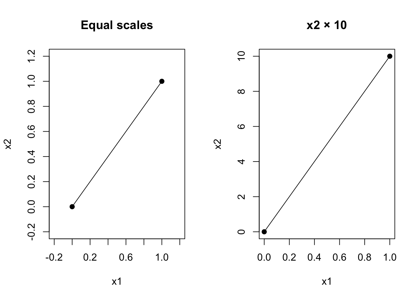
| Data type | Possible dissimilarity | Important question |
|---|---|---|
| Continuous numerical | Euclidean or Manhattan | Are scale differences meaningful? |
| Nominal categories | Simple matching | Are all mismatches equally different? |
| Asymmetric binary | Jaccard | Should shared absences count? |
| Mixed types | Gower | How should types be combined? |
| Text / embeddings | Cosine | Does direction matter more than magnitude? |
This exam’s coding uses numerical features and Euclidean distance. The table is for theory questions that ask whether a measure is appropriate.
The silhouette needs a fitted partition. It appears in the k-means chapter after Lloyd’s algorithm has produced clusters.
Two clinics are compared on age and blood pressure. Blood pressure is recorded in mmHg (roughly 80–180) and age in years (roughly 20–90). Without scaling, which feature tends to dominate Euclidean distance, and why?
For \mathbf{x}_1=(1,1) and \mathbf{x}_2=(4,5), state d_E and d_M.