a <- c(1, 2, 2) / 3
x <- c(2, -1, 3)
Sigma <- matrix(c(1, 0.5, 0.25, 0.5, 1, 0.5, 0.25, 0.5, 1), 3, 3)
c(score = sum(a * x), variance = as.numeric(t(a) %*% Sigma %*% a))
score variance
2.000000 1.777778 Study time: about 3 hours. Calculations plus prcomp. Later methods are defined against PCA.
You have p numerical variables and want fewer new variables that still separate observations. PCA builds each new variable as a linear combination of the originals:
a_1 x_1 + \cdots + a_p x_p.
There is no response label — the method is unsupervised.
For a unit vector \mathbf{a} and observation \mathbf{x}, the score is y=\mathbf{a}'\mathbf{x}. Without a fixed length, multiplying \mathbf{a} by a constant would inflate the variance of y without changing the direction. Unit length is convenient: then \operatorname{Var}(Y)=\mathbf{a}'\boldsymbol{\Sigma}\mathbf{a} equals the corresponding eigenvalue when \mathbf{a} is an eigenvector.
With mean-zero \mathbf{X} and covariance \boldsymbol{\Sigma},
\mathbf{a}_1=\arg\max_{\mathbf{a}'\mathbf{a}=1}\mathbf{a}'\boldsymbol{\Sigma}\mathbf{a}.
Later components maximise the same objective subject to orthogonality to earlier loadings. Without orthogonality, every component would pick the same direction as the first.
The solution is the eigenvector sequence of \boldsymbol{\Sigma}: Y_i=\mathbf{e}_i'\mathbf{X}, \operatorname{Var}(Y_i)=\lambda_i, and distinct components are uncorrelated. Total variance is preserved:
\sum_j\operatorname{Var}(X_j)=\sum_i\lambda_i.
Proportion explained by component k: \lambda_k/\sum_i\lambda_i.
Centred and standardised \mathbf{x}=(2,-1,3)' with \mathbf{a}_1=\bigl(\tfrac13,\tfrac23,\tfrac23\bigr)':
y_1=\tfrac13\cdot 2+\tfrac23\cdot(-1)+\tfrac23\cdot 3=2.
Same \mathbf{a} with
\boldsymbol{\Sigma}= \begin{pmatrix} 1 & 0.5 & 0.25\\ 0.5 & 1 & 0.5\\ 0.25 & 0.5 & 1 \end{pmatrix}
gives \mathbf{a}'\boldsymbol{\Sigma}\mathbf{a}=16/9.
a <- c(1, 2, 2) / 3
x <- c(2, -1, 3)
Sigma <- matrix(c(1, 0.5, 0.25, 0.5, 1, 0.5, 0.25, 0.5, 1), 3, 3)
c(score = sum(a * x), variance = as.numeric(t(a) %*% Sigma %*% a)) score variance
2.000000 1.777778 PCA on the covariance matrix lets large-scale variables dominate. Standardise (scale. = TRUE in prcomp) when equal numerical influence matches the question. Height and weight in different units: standardise. Gene expression with near-zero-variance unexpressed genes: do not blindly standardise noise — exclude or transform first.
A flat scree plot suggests comparable variances and weak correlations — little low-dimensional linear structure.
If PC1 explains ~99% and loads on one variable, that variable’s scale or variance likely dominates.
Multiplying a loading vector by -1 leaves the axis the same. The verbal summary (“overall size”) is unchanged; score signs flip.
X <- scale(USArrests)
pca <- prcomp(USArrests, center = TRUE, scale. = TRUE)
summary(pca)
Importance of components:
PC1 PC2 PC3 PC4
Standard deviation 1.5749 0.9949 0.59713 0.41645
Proportion of Variance 0.6201 0.2474 0.08914 0.04336
Cumulative Proportion 0.6201 0.8675 0.95664 1.00000plot(pca$x[, 1], pca$x[, 2], pch = 19,
xlab = "PC1", ylab = "PC2", main = "USArrests PCA")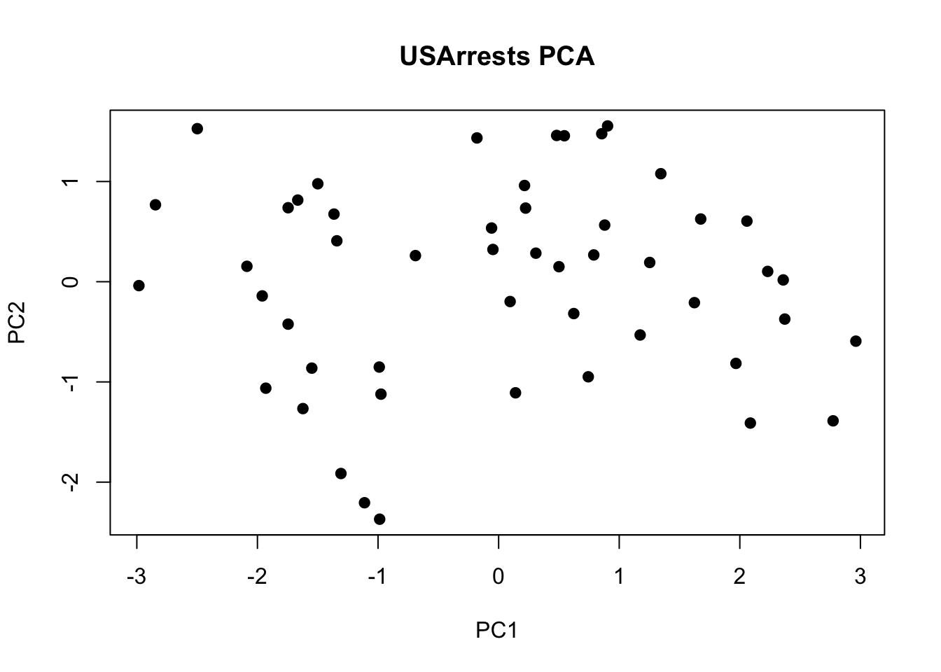
# Loadings
round(pca$rotation[, 1:2], 3)
PC1 PC2
Murder -0.536 -0.418
Assault -0.583 -0.188
UrbanPop -0.278 0.873
Rape -0.543 0.167Interpretation habit. Name PC1 by which variables have large loadings (e.g. overall crime versus UrbanPop). Do not recite every coefficient.
PCA only finds linear subspaces. A Swiss roll needs a non-linear method (ISOMAP, non-linear autoencoder).
prcomp and eigen on the same matrix agree up to sign flips of eigenvectors.Why restrict loadings to unit length? Is unit length special?
Problem with simply maximising variance for each component?
\mathbf{x}=(2,-1,3)', \mathbf{a}_1=(1/3,2/3,2/3)'. Score?
Same \mathbf{a} and \boldsymbol{\Sigma} as above. Variance?