Study time: about 2 hours. Input is a dissimilarity matrix; output is a low-dimensional map.
5.1 Pass
5.1.1 Situation
PCA needs a feature matrix. Sometimes you only have pairwise dissimilarities — cities by road time, documents by a custom distance, binary data with Jaccard. MDS places points in k dimensions so that map distances track those dissimilarities.
A k-dimensional map has kn free coordinates (2n when k=2).
5.1.2 Three distances
\delta_{ij}: supplied dissimilarity (the input).
d_{ij}=\|\mathbf{y}_i-\mathbf{y}_j\|: Euclidean distance between fitted map points.
\hat{d}_{ij}=f(\delta_{ij}): disparity — the target distance after a fitted transformation in non-metric MDS.
5.1.3 Classical MDS
Classical MDS recovers coordinates from a centred inner-product matrix built from the dissimilarities (double centring), then an eigendecomposition — the same linear-algebra step as PCA when the dissimilarities are Euclidean distances from a feature matrix.
Aim in one line: represent centred inner products (course answer). Orientation of the plot is arbitrary: rotation and reflection leave interpoint distances unchanged.
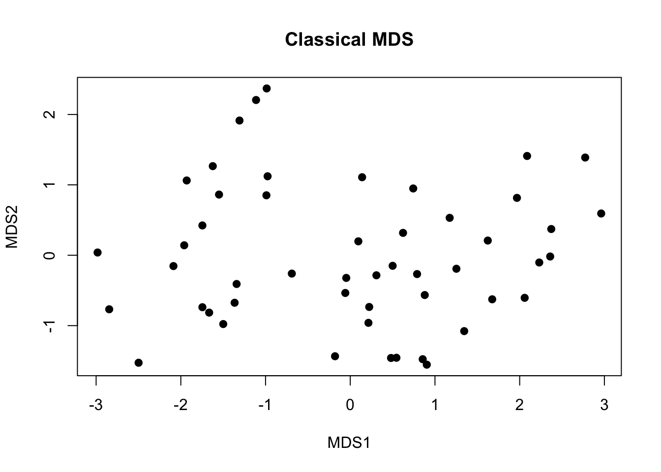
X <-scale(USArrests)d <-dist(X)mds <-cmdscale(d, k =2, eig =TRUE)plot(mds$points, pch =19, xlab ="MDS1", ylab ="MDS2",main ="Classical MDS")
Classical MDS on scaled USArrests (Euclidean).
# Rough analogue of variance explained: positive eigenvaluesround(mds$eig[1:4], 3)
[1] 121.532 48.498 17.472 8.498
When \delta_{ij} are Euclidean distances from features, classical MDS and PCA give the same configuration up to rotation/reflection.
5.1.4 Metric least-squares and weights
Metric MDS can minimise a weighted sum of squared errors between d_{ij} and \delta_{ij}. Weights that shrink as \delta_{ij} grows give more priority to small dissimilarities. The map distances still aim at the numerical dissimilarities; only which errors matter most changes.
5.1.5 Non-metric MDS
Only the rank order of dissimilarities is treated as meaningful. Stress measures how poorly the map preserves that order (monotone relationship between \delta_{ij} and d_{ij}). Interpret order, not raw length ratios.
MASS::sammon is a related metric stress with denominator \delta_{ij} (prac contrast). Classical cmdscale remains the default exam call.
5.1.6 Scaling and suitability
Standardise features before Euclidean distances when equal influence is intended — same logic as clustering and PCA.
MDS suits binary or mixed data better when you can choose a specialised \delta_{ij}. PCA on 0/1 columns is not always wrong, but it forces a Euclidean/feature view.
MDS stores all pairs: O(n^2) cost. Painful for large n.
5.2 Reference
Shepard diagram: plot d_{ij} (or \hat{d}_{ij}) against \delta_{ij} to see fit.
Choose k by eigenvalue scree of classical MDS or by stress curves for iterative MDS.
Practical workflow: choose dissimilarity → classical MDS → inspect map and fit → try non-metric only if ranks matter more than magnitudes.
5.3 Recall
Official — parameters
How many parameters for a 2-D map? For a k-D map?
Answer
2n and kn: one coordinate per observation per map dimension.