Study time: about 3.5 hours. About 20 of the 30 clustering written marks, plus 10 coding marks. This was not on the class test — prioritise it.
3.1 Pass
3.1.1 Nested clusters and the dendrogram
Some questions ask for a taxonomy: small groups inside larger groups. Agglomerative hierarchical clustering builds that taxonomy from the bottom up.
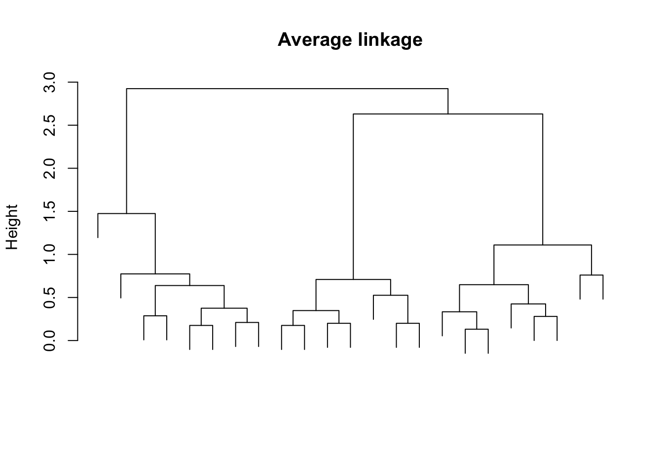
Start with every observation alone. Repeatedly merge the two closest clusters until one cluster remains. The record of merges is a dendrogram: height marks the dissimilarity at which a merge happened. Horizontal spacing in the plot is layout, not distance.
Once two clusters merge, they never separate at higher levels. Early merge mistakes propagate. The fit itself is deterministic for a fixed dissimilarity and linkage — no seed, no nstart.
Cutting the tree at a height, or asking for K groups with cutree, yields a partition you can silhouette and profile exactly as in k-means.
Same numbers, three answers. For d(3,1)=0.22 and d(6,1)=0.23,
Linkage
d(\{3,6\},\{1\})
Single
\min(0.22,0.23)=0.22
Complete
\max(0.22,0.23)=0.23
Average
\frac{1}{2}(0.22+0.23)=0.225
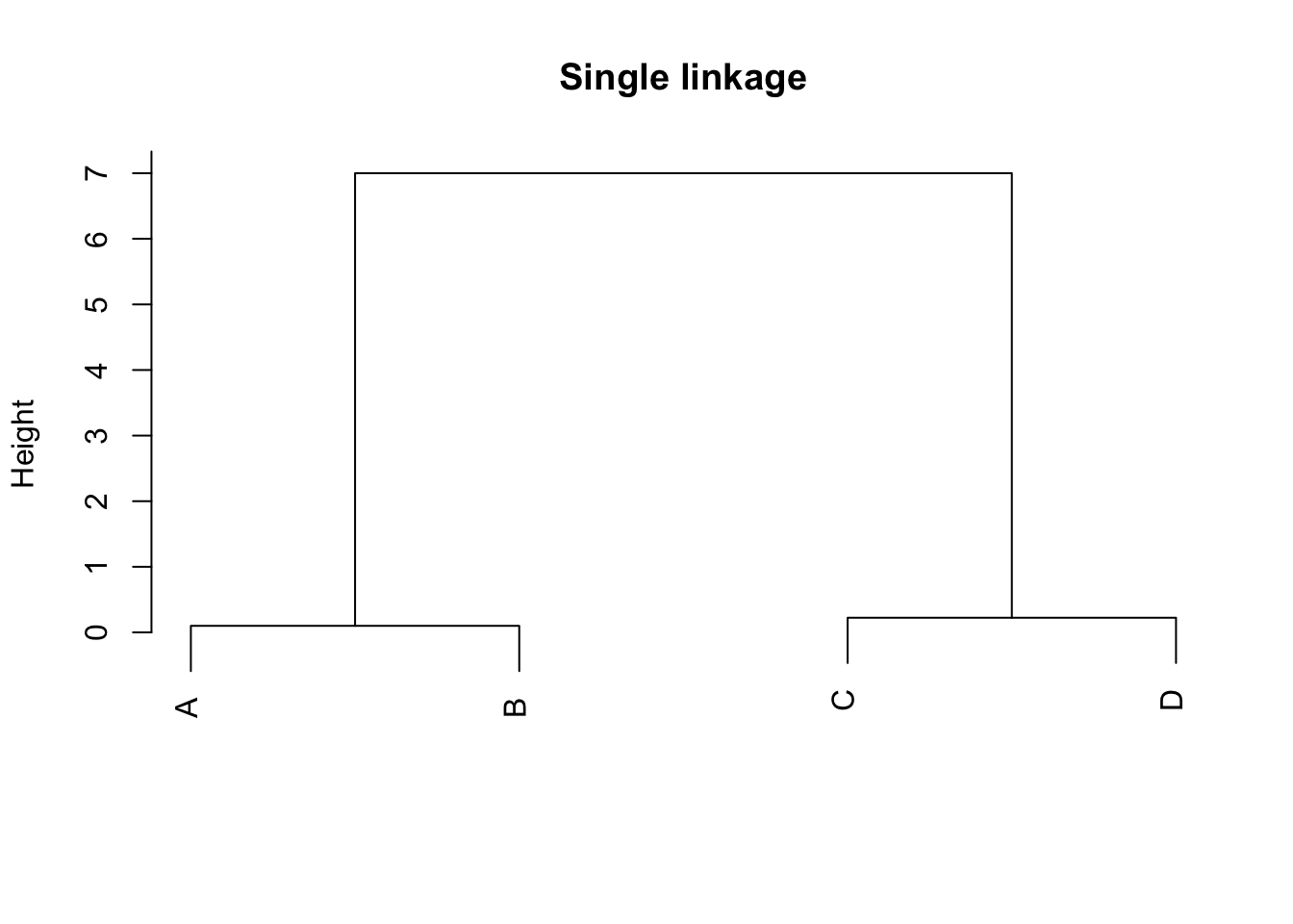
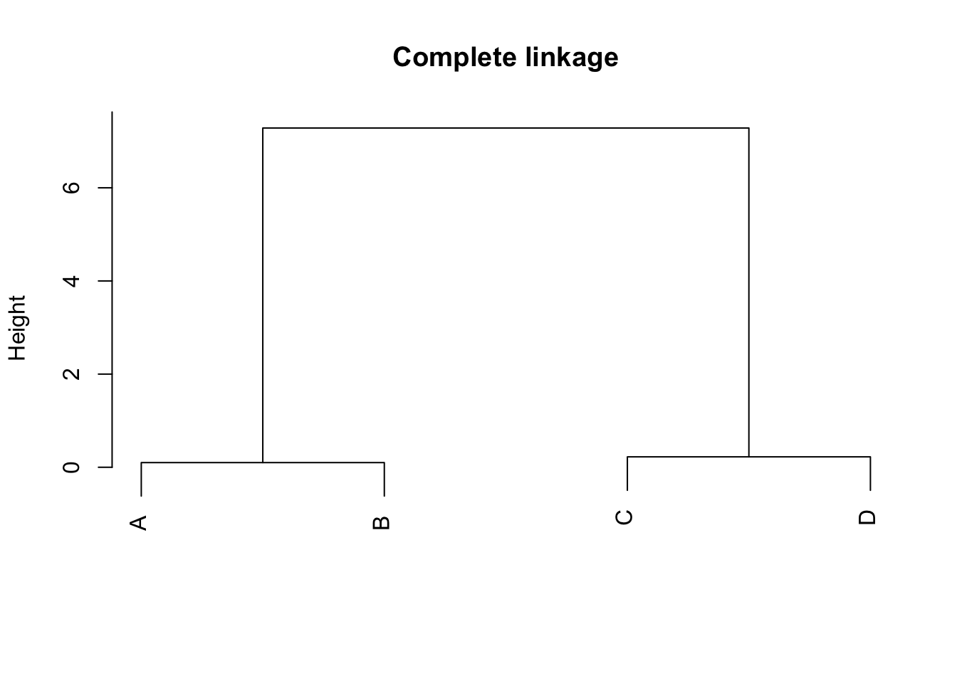
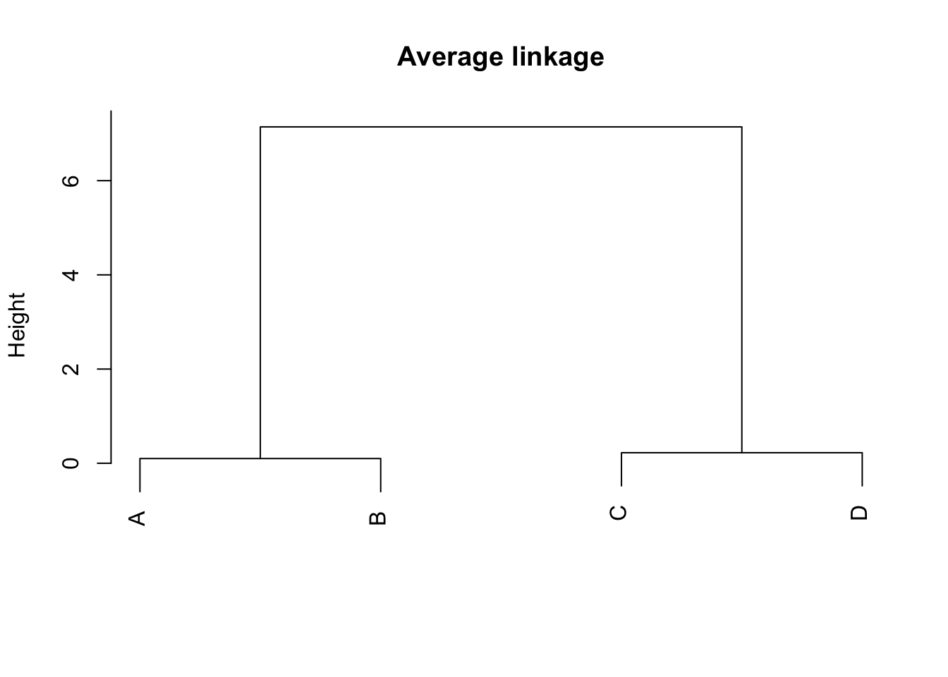
Single can chain through a bridge point: one close pair is enough to merge elongated shapes. Complete waits until every pair between groups is close enough, so clusters tend to be more compact and balanced. Average is a compromise with a clear “mean pairwise gap” reading.
3.1.3 Interactive check: same distances, three trees
# Four points: two tight pairs far apartpts <-matrix(c(0, 0, 0.1, 0, 5, 5, 5.1, 5.2), ncol =2, byrow =TRUE)rownames(pts) <-c("A", "B", "C", "D")d <-dist(pts)d
          A         B         C
B 0.1000000
C 7.0710678 7.0007142
D 7.2835431 7.2138755 0.2236068
Mechanism. The smallest entry is d(A,B)=2, so merge \{A,B\} first at height 2. Complete linkage distance from \{A,B\} to C is \max(6,5)=6; to D is \max(10,9)=10. Next smallest among remaining is d(C,D)=4, so merge \{C,D\} at height 4. Final merge height is \max of all cross pairs between \{A,B\} and \{C,D\}, which is 10. Cutting to K=2 recovers the two pairs.
3.1.5 Judging a cut
Reuse silhouette, negative counts, subsample stability, and profiles from the k-means workflow. Extra hierarchical facts:
Merge-height gaps can suggest K native to the tree.
Silhouette and merge gaps can disagree — shortlist both, then decide with purpose.
Single linkage’s highest silhouette can be a useless “one outlier vs the rest” split. Prefer a linkage whose profiles match the decision, and report the weaker silhouette if that is the tradeoff.
Subsampling still matters: the algorithm is deterministic on a fixed sample, but the sample can change.
3.1.6 Commands from memory
x <-scale(as.matrix(df[, numeric_cols]))d <-dist(x, method ="euclidean")hc <-hclust(d, method ="average") # or "single" / "complete"plot(hc)groups <-cutree(hc, k =3)sil <- cluster::silhouette(groups, d)mean(sil[, "sil_width"])
Compare linkages on the samedist object. Do not rebuild distances differently between methods unless the question asks for that.
3.1.7 Lab rhythm (uns scaffolded)
On the toy routes file:
Scale if equal influence is intended; form dist.
Fit single, complete, average; plot dendrograms.
Shortlist K with silhouette and merge gaps.
Inspect weak silhouettes; compare two linkages with table().
Profile means; recommend, revise, or reject with one evidence line and one limitation.
Average-linkage dendrogram on the hierarchical toy routes.
groups <-cutree(hc, k =3)table(groups)
groups
1 2 3
7 8 8
3.2 Reference
Horizontal cut at a height h keeps merges below h and splits merges above h.
Dendrogram height is in dissimilarity units of the input matrix, not raw feature units unless those coincide.
Monotone transformation of all dissimilarities can change average linkage (means use the numbers) while leaving the order of single/complete merges unchanged if the order of pairwise distances is preserved — the exercise set probes this.
Hierarchical vs k-means: one tree vs many random starts; any dissimilarity vs squared Euclidean on features; final merges vs revisable assignments.
3.3 Recall
Official-style — single linkage definition
For clusters G and H, single-linkage dissimilarity is…
Answer
The minimum pairwise dissimilarity between a point in G and a point in H. Reason: “closest members” rule.
Official — B1 pattern (complete hierarchy)
Using the four-point complete-linkage matrix above, state the first merge height and the K=2 partition.
Answer
First merge \{A,B\} at height 2. At K=2: \{A,B\} and \{C,D\}. Reason: smallest pairwise distance merges first; complete linkage then uses maxima between groups.
Official-style — chaining
GPS tracks form elongated routes; a few isolated errors remain. Why is single linkage risky?
Answer
One bridge point (or error) can link distinct routes because only the minimum cross distance matters. Prefer average or complete when compact programme groups are required.
Official-style — silhouette vs purpose
Single linkage K=2 has higher average silhouette than average linkage K=3, but K=2 merely separates salinity extremes while the brief asks for multivariate handling profiles. Strongest conclusion?
Answer
Prefer average linkage at K=3 provisionally if it matches the stated purpose; report the weaker silhouette and validate. Largest silhouette is not an automatic override of the decision question.
Original — deterministic fit
Why does hierarchical clustering need no nstart?
Answer
For fixed dissimilarities and linkage, each merge is determined by the linkage rule. Random initialisation is not part of the algorithm. Sensitivity still appears through the sample and the linkage choice.