8  Autoencoders

Study time: about 2 hours. Coding: know the main calls, extract the latent layer, interpret reconstruction — no simulation loops.

8.1 Pass

8.1.1 Situation

You want a low-dimensional code that can rebuild the input. An autoencoder is a neural net trained to predict its own inputs.

• Encoder: maps input \mathbf{x} to the code \mathbf{z} (bottleneck).
• Decoder: maps \mathbf{z} back toward \mathbf{x}.
• Bottleneck: narrowest layer; the latent representation.

If the bottleneck is as wide as the input, there is no compression — the net can learn to copy.

8.1.2 Loss and activations

The target is the input (or a clean input, for denoising). Squared error suits continuous features; binary cross-entropy suits binary features.

Non-linear activations matter: with only linear layers and squared error, the model spans the same subspace as PCA (up to rotation) and does not even order components by variance. Non-linearity is what buys curved manifolds.

8.1.3 Overfitting and held-out data

The architecture is flexible. Held-out validation/test data are required to see whether reconstruction generalises. Early stopping uses validation loss.

Reconstruction error on training data can rise with a wider bottleneck if a larger net was not trained long enough. On test data, rising error with width often signals overfitting.

8.1.4 Denoising

Input: corrupted \mathbf{x} (noise, or variables zeroed). Target: clean \mathbf{x}. Forces robustness and discourages trivial copying.

8.1.5 MNIST lesson (prose only)

A linear output layer is natural for unbounded reconstructions; clip only for display. A ReLU bottleneck forces non-negative codes. Reconstruction MSE can look excellent because most pixels are background white — still check whether digits are confused.

8.1.6 Runnable: keras3 on iris (this year’s verbs)

library(reticulate)
use_virtualenv("r-keras", required = TRUE)
library(keras3)

x <- scale(as.matrix(iris[, 1:4]))
set.seed(5077)
tensorflow::set_random_seed(5077)

model <- keras_model_sequential(input_shape = ncol(x)) |>
  layer_dense(units = 8, activation = "relu") |>
  layer_dense(units = 2, activation = "linear", name = "bottleneck") |>
  layer_dense(units = 8, activation = "relu") |>
  layer_dense(units = ncol(x))

model |> compile(loss = "mean_squared_error", optimizer = "adam")
model |> fit(x, x, epochs = 80, batch_size = 16, verbose = 0, validation_split = 0.2)

encoder <- keras_model(
  inputs = model$inputs,
  outputs = get_layer(model, "bottleneck")$output
)
z <- predict(encoder, x, verbose = 0)
plot(z[, 1], z[, 2], col = as.integer(iris$Species), pch = 19,
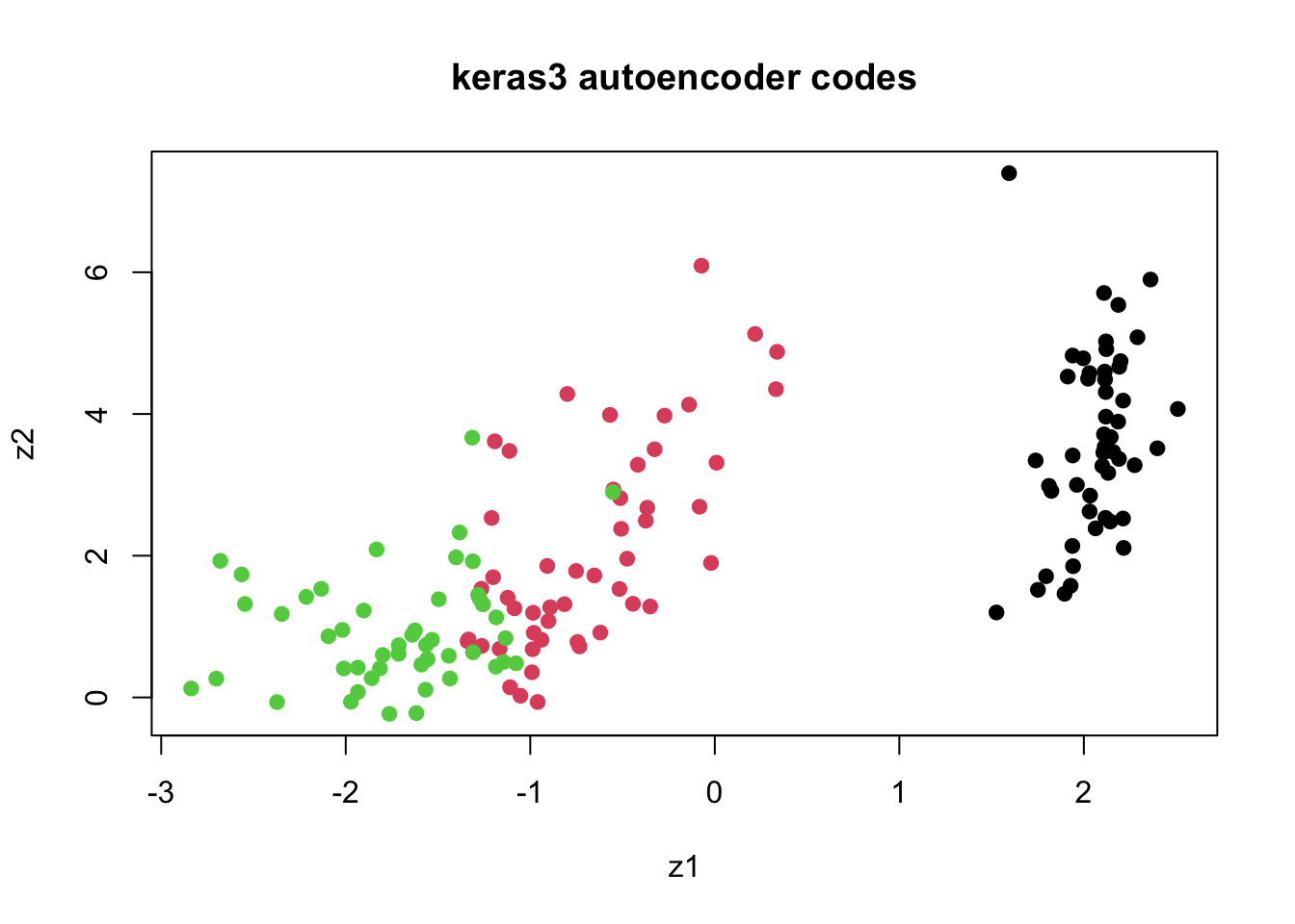
     xlab = "z1", ylab = "z2", main = "keras3 autoencoder codes")

Iris: 2-D bottleneck codes coloured by species (species not used in training).

recon <- predict(model, x, verbose = 0)
mse <- mean((x - recon)^2)
mse

[1] 0.06924728

8.1.7 Runnable: h2o pattern (last year’s fill-in)

library(h2o)
h2o.init(nthreads = 2, max_mem_size = "2G")

H2O is not running yet, starting it now...

Note:  In case of errors look at the following log files:
    /var/folders/b4/q35h60c10_53lf20j68vwbd00000gn/T//RtmpKt2m6Z/filee685d7054d5/h2o_maesela_started_from_r.out
    /var/folders/b4/q35h60c10_53lf20j68vwbd00000gn/T//RtmpKt2m6Z/filee6879d19bdf/h2o_maesela_started_from_r.err


Starting H2O JVM and connecting: .. Connection successful!

R is connected to the H2O cluster: 
    H2O cluster uptime:         2 seconds 64 milliseconds 
    H2O cluster timezone:       Africa/Johannesburg 
    H2O data parsing timezone:  UTC 
    H2O cluster version:        3.44.0.3 
    H2O cluster version age:    2 years, 10 months and 19 days 
    H2O cluster name:           H2O_started_from_R_maesela_lxv521 
    H2O cluster total nodes:    1 
    H2O cluster total memory:   1.98 GB 
    H2O cluster total cores:    10 
    H2O cluster allowed cores:  2 
    H2O cluster healthy:        TRUE 
    H2O Connection ip:          localhost 
    H2O Connection port:        54321 
    H2O Connection proxy:       NA 
    H2O Internal Security:      FALSE 
    R Version:                  R version 4.5.3 (2026-03-11) 

iris_feat <- as.data.frame(scale(iris[, 1:4]))
iris_h2o <- as.h2o(iris_feat)

  |                                                                            
  |                                                                      |   0%
  |                                                                            
  |======================================================================| 100%

ae <- h2o.deeplearning(
  x = names(iris_feat),
  training_frame = iris_h2o,
  autoencoder = TRUE,
  hidden = c(8, 2, 8),
  activation = "Tanh",
  epochs = 50,
  reproducible = TRUE,
  seed = 5077
)

  |                                                                            
  |                                                                      |   0%
  |                                                                            
  |======================================================================| 100%

latent <- as.data.frame(h2o.deepfeatures(ae, iris_h2o, layer = 2))

  |                                                                            
  |                                                                      |   0%
  |                                                                            
  |======================================================================| 100%

plot(latent[[1]], latent[[2]], col = as.integer(iris$Species), pch = 19,
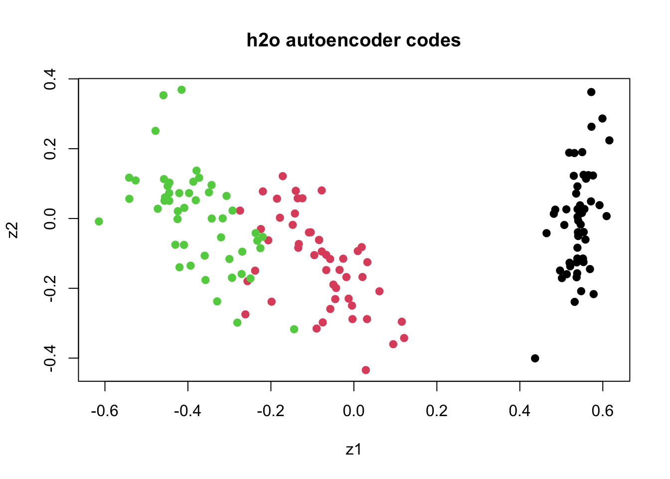
     xlab = "z1", ylab = "z2", main = "h2o autoencoder codes")

Iris: h2o deepfeatures at the bottleneck layer.

pred <- as.data.frame(h2o.predict(ae, iris_h2o))

  |                                                                            
  |                                                                      |   0%
  |                                                                            
  |======================================================================| 100%

mse_h2o <- mean((as.matrix(iris_feat) - as.matrix(pred))^2)
mse_h2o

[1] 0.04989139

h2o.shutdown(prompt = FALSE)

Architecture hidden = c(10, 2, 10) means encode p\to 10\to 2, then decode 2\to 10\to p. The middle 2 is the bottleneck code.

8.2 Reference

• Compare latent scatter to PCA on the same scaled features: species separation can differ because of non-linearity.
• Linear autoencoder \approx PCA subspace, possibly rotated; components need not be ordered by variance.
• Choosing latent dimension: watch train and validation reconstruction curves.

8.3 Recall

Official — encoder / decoder / bottleneck

Roles?

Answer

Encoder → code; bottleneck holds the code; decoder reconstructs toward the input space.

Official — like PCA when?

When does an autoencoder behave like PCA?

Answer

When activations are linear (squared-error training): same subspace, possible rotation.

Official — denoising

Input and target? Why?

Answer

Input corrupted; target clean original. Builds robustness and blocks trivial identity maps.

Official — held-out data

Why required?

Answer

Flexible models overfit; need validation/test reconstruction to judge generalisation.