11  Blank exam rehearsal

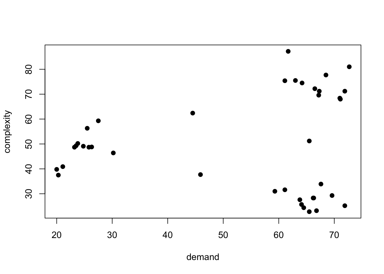
Closed-book. Type MCQ letters and short answers as plain text. Put code in the chunks. Do not open other chapters.

Mark guide (matches the lecturers’ split): Clustering 50 · DR 50. Clustering theory ≈ 30 (about two-thirds hierarchical) · clustering code ≈ 20 (10 k-means + 10 hierarchical). DR theory ≈ 25–30 · DR code ≈ 20–25.

12 Section A — Clustering [50]

12.1 Theory [~30]

About two-thirds of these are hierarchical. For MCQs, write only the letter.

12.1.1 A1 (MCQ)

Which statement best describes the main aim of k-means clustering?

A. Find K representative observations that minimise total dissimilarity to the other observations assigned to their clusters.
B. Find assignments and centroids that minimise the within-cluster sum of squares.
C. Find K representatives that minimise the largest distance from any observation to its representative.
D. Merge the closest pair of clusters repeatedly until exactly K clusters remain.

Answer:

12.1.2 A2 (MCQ)

What happens in the assignment step of Lloyd’s k-means algorithm?

A. Each observation is allocated to its nearest current centroid.
B. Each observation is allocated to the cluster whose current members have the smallest average dissimilarity to it.
C. Each centroid is replaced by the coordinate-wise mean of its currently assigned observations.
D. The cluster with the largest WCSS is given a new randomly chosen centroid.

Answer:

12.1.3 A3 (MCQ)

An observation has a negative silhouette value. What does this most directly indicate?

A. Its own cluster is closer on average than the nearest alternative cluster, but only by a small amount.
B. Its assigned cluster has a larger average WCSS than the other fitted clusters.
C. Its nearest alternative cluster is closer on average than its assigned cluster.
D. Its squared distance to its centroid is above the average squared distance in its cluster.

Answer:

12.1.4 A4 (MCQ)

Which statement best describes agglomerative hierarchical clustering?

A. Start with one cluster and repeatedly split the cluster with largest WCSS until K clusters remain.
B. Start with each observation alone and repeatedly merge the closest pair of clusters until one cluster remains.
C. Alternate assignment and centroid update until assignments stop changing.
D. Assign each observation to the nearest of K randomly chosen medoids.

Answer:

12.1.5 A5 (MCQ)

For clusters G and H, how is single-linkage dissimilarity defined?

A. The maximum pairwise dissimilarity between a point in G and a point in H.
B. The minimum pairwise dissimilarity between a point in G and a point in H.
C. The average of all pairwise dissimilarities within G and within H.
D. The dissimilarity between the two cluster centroids.

Answer:

12.1.6 A6 (MCQ)

A property of agglomerative hierarchical clustering is that

A. merges can be undone if a better split is found later.
B. the dendrogram height has the same units as the original data matrix.
C. once two clusters are merged, they never separate at higher levels.
D. it always reproduces the k-means partition when cut at K.

Answer:

12.1.7 A7 (MCQ)

GPS tracks form elongated routes; a few isolated GPS errors may remain. Which assessment of single linkage is best?

A. Prefer single linkage because it always maximises average silhouette.
B. Single linkage is attractive for elongated shapes but is sensitive to bridge points and noise; average or complete may be safer for compact programmes.
C. Single linkage is immune to outliers because it uses the maximum cross distance.
D. Single and complete linkage always give the same dendrogram on Euclidean distances.

Answer:

12.1.8 A8 (MCQ)

Why is a visible bend in an elbow plot not proof that the data contain natural clusters?

A. The elbow is always at K=2.
B. A bend becomes formal evidence only after averaging WCSS over enough random starts.
C. WCSS falls mechanically as K grows, and even structureless data can produce a bend.
D. The elbow requires the true number of clusters as input.

Answer:

12.1.9 A9 (short answer, ~3 marks)

Six observations, K=2. Start with centroids \boldsymbol{\mu}_1=(1,1) and \boldsymbol{\mu}_2=(7,7).

Obs	x_1	x_2
A	1	1
B	1	2
C	2	1
D	7	7
E	8	7
F	7	8

1. Assign each observation to its nearest centroid.
   
2. Calculate the two updated centroids.

Answer:

12.1.10 A10 (short answer, ~3 marks)

For one observation, a(i)=1.20 and b(i)=1.50.

1. Calculate its silhouette value.
   
2. Interpret the value in one sentence.
   
3. State one sensible follow-up check.

Answer:

12.1.11 A11 (short answer, ~4 marks)

Dissimilarities: d(A,B)=2, d(A,C)=6, d(A,D)=10, d(B,C)=5, d(B,D)=9, d(C,D)=4. Use complete linkage.

1. Which pair merges first, and at what height?
   
2. After that merge, what is the complete-linkage distance from the new cluster to C? To D?
   
3. List the clustering obtained by cutting the completed dendrogram at K=2.

Answer:

12.1.12 A12 (short answer, ~4 marks)

A team wants multivariate handling profiles for shipment routes. Single linkage at K=2 has average silhouette 0.54 but mainly separates one salinity extreme. Average linkage at K=3 has silhouette 0.43 and three distinct operational profiles.

Give a verdict: recommend / revise / reject. Support with purpose, fit or stability, usefulness, and one limitation.

Answer:

12.2 Coding [~20]

12.2.1 K-means (~10)

lab <- read.csv("data/kmeans-lab-toy.csv")
x_raw <- as.matrix(lab[, c("demand_score", "complexity_score")])
plot(x_raw, pch = 19, xlab = "demand", ylab = "complexity")

1. Decide whether to standardise. Justify in one or two sentences, then prepare the matrix you will cluster.
   
2. Fit k-means for K=3 with nstart = 25 and a fixed seed. Report tot.withinss and cluster sizes.
   
3. Using dist and cluster::silhouette, compute the mean silhouette for K=2,3,4,5. State which K you prefer and why (one or two sentences).
   
4. For your preferred fit, name one variable pattern that characterises each cluster (interpretation).

# Your clustering code

Interpretation:

12.2.2 Hierarchical (~10)

routes <- read.csv("data/hierarchical-clustering-lab-toy.csv")
num <- routes[sapply(routes, is.numeric)]
plot(num[, 1:2], pch = 19)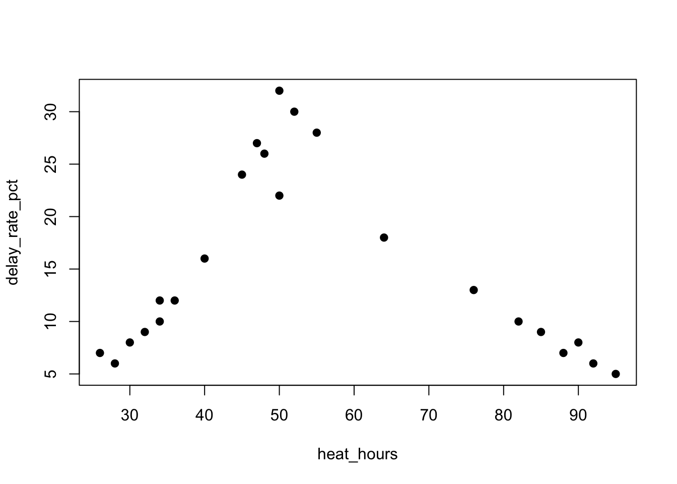

1. Scale the numeric features if appropriate; form a Euclidean dist object.
   
2. Fit single, complete, and average linkage; plot the three dendrograms.
   
3. For complete and average, compute average silhouette for K=2,3,4. Shortlist one linkage and one K.
   
4. Cut your preferred tree; report sizes; interpret each cluster in one short phrase.
   
5. Compare your preferred groups to complete linkage at the same K using table(). Comment in one sentence.

# Your clustering code

Interpretation:

12.2.3 Recovery practice

# If a chunk fails in the real exam: set eval: false or hand in the source.
# That recovers rendering — it does not replace the answer.
stop("example failure")

13 Section B — Dimension reduction [50]

13.1 Theory [~25–30]

13.1.1 B1 (MCQ)

You have performed PCA on a dataset with 50 features. The first 5 principal components explain 99% of the cumulative variance. What is the most plausible conclusion?

A. The original data likely contained a high degree of multicollinearity.
B. The original 50 features were all standardized to have a mean of 0.
C. The data lies almost entirely on a 5-dimensional linear subspace within the original 50-dimensional space.
D. The PCA analysis was run incorrectly, as this result is statistically impossible.

Answer:

13.1.2 B2 (MCQ)

In non-metric MDS, “stress” primarily measures:

A. The total variance in the original high-dimensional data.
B. The degree to which the rank-order of distances in the low-dimensional plot is preserved compared to the original dissimilarities.
C. The sum of squared errors between the original data points and their projections.
D. The correlation between the original variables and the MDS dimensions.

Answer:

13.1.3 B3 (MCQ)

The ISOMAP algorithm fundamentally differs from PCA by:

A. Using a different optimization criterion for eigenvalue decomposition.
B. Approximating geodesic distances along the data manifold rather than Euclidean distances.
C. Employing a neural network architecture for non-linear projections.
D. Requiring categorical variables to be one-hot encoded.

Answer:

13.1.4 B4 (MCQ)

During SOM training, the primary purpose of the neighbourhood function is:

A. To determine the initial random weights of the output nodes.
B. To define the learning rate schedule for the entire network.
C. To update not only the BMU but also its topological neighbours, preserving topology.
D. To calculate the quantization error of the final map.

Answer:

13.1.5 B5 (MCQ)

When comparing PCA to linear autoencoders with squared error loss under optimal training:

A. The autoencoder bottleneck learns different components than PCA.
B. The autoencoder learns non-orthogonal components while PCA learns orthogonal ones.
C. The autoencoder bottleneck learns the same subspace as PCA but may rotate it.
D. Autoencoders cannot learn linear projections comparable to PCA.

Answer:

13.1.6 B6 (short answer)

Why must a PCA loading vector be restricted to unit length? Is unit length special compared with any other fixed length?

Answer:

13.1.7 B7 (short answer)

Calculate the principal component score for centred standardised \mathbf{x}=(2,-1,3)' and \mathbf{a}_1=\bigl(\frac13,\frac23,\frac23\bigr)'.

Answer:

13.1.8 B8 (short answer)

Contrast \delta_{ij}, d_{ij} and \hat{d}_{ij} in MDS notation.

Answer:

13.1.9 B9 (short answer)

Discuss the effect on the k-nearest-neighbour graph and the ISOMAP embedding of setting k=1 and k=n-1. What is a reasonable middle ground?

Answer:

13.1.10 B10 (short answer)

1. Does a SOM node with no allocated observations still have a prototype? How is it determined?
   
2. What is quantisation error? What is topographic error? How do they complement each other?

Answer:

13.1.11 B11 (short answer)

1. Role of the encoder and of the decoder?
   
2. In a denoising autoencoder, what is the input and what is the target? Why?

Answer:

13.1.12 B12 (short answer / calculation)

SOM update: \alpha_t=0.5, \mathbf{x}_i-\mathbf{m}_j=(0.4,-0.1)', \boldsymbol{\ell}_{b_i}=(1,2)', \boldsymbol{\ell}_j=(5,5)', h=\exp(-\|\boldsymbol{\ell}_{b_i}-\boldsymbol{\ell}_j\|^2/(2\sigma^2)). Find \sigma^2 so that \Delta\mathbf{m}_j=(0.1,-0.025)'.

Answer:

13.2 Coding [~20–25]

Data already in memory:

X <- scale(USArrests)

13.2.1 PCA (~6)

1. Fit PCA with prcomp on USArrests with centring and scaling.
   
2. What cumulative proportion of variance do PC1 and PC2 explain together?
   
3. Interpret PC1 from the loadings: crime vs urbanisation? Justify.

# Your code

Interpretation:

13.2.2 MDS (~5)

1. Why is standardising critical before Euclidean distances here?
   
2. Compute the Euclidean distance matrix from X.
   
3. Fit classical MDS in 2-D with cmdscale.
   
4. Comment briefly on how high-crime/urban states sit relative to low-crime rural states on the map.

# Your code

Interpretation:

13.2.3 ISOMAP (~7)

Use the Swiss-roll style point cloud below (already generated). Fit ISOMAP for k=5, k=15, and k=30 (either vegan::isomap or Rdimtools::do.isomap). Plot the embeddings. Which k unfolds best, and why does PCA fail here?

set.seed(5077)
n <- 400
t <- runif(n, 0, 3 * pi)
h <- runif(n, 0, 20)
swiss <- cbind(x = t * cos(t), y = h, z = t * sin(t))

# Your code

Interpretation:

13.2.4 Autoencoder (~7)

On scaled iris[, 1:4] (species unused in training):

1. Fit a small autoencoder with a 2-D bottleneck (keras3 or h2o).
   
2. Extract the 2-D codes and plot them.
   
3. Report reconstruction MSE.
   
4. In two sentences, compare the latent scatter to a 2-D PCA of the same features.

# Your code

Interpretation: