Study time: about 2.5 hours. About 10 written marks and 10 coding marks. PAM / k-medoids: not examinable (slides 24–32).
2.1 Pass
2.1.1 The objective
You want K groups of numerical observations. K-means seeks assignments C(i)\in\{1,\ldots,K\} and centroids \boldsymbol{\mu}_1,\ldots,\boldsymbol{\mu}_K that minimise the within-cluster sum of squares (WCSS):
Each term is squared Euclidean distance from a point to its own centroid. That is why feature scale matters: a stretched coordinate inflates those squares.
2.1.2 Lloyd’s algorithm
The objective is hard to minimise jointly. Lloyd’s algorithm alternates two cheaper steps:
Assign: give each observation to its nearest current centroid.
Update: replace each centroid by the coordinate-wise mean of its assigned observations.
Repeat until assignments stop changing. The WCSS never increases at either step, but the path can stop at a local optimum. Different starting centroids can give different partitions and different WCSS values.
# Six points, K = 2, start at A and D (course exercise)pts <-matrix(c(1, 1, 1, 2, 2, 1, 7, 7, 8, 7, 7, 8),ncol =2, byrow =TRUE,dimnames =list(LETTERS[1:6], c("x1", "x2")))mu <- pts[c("A", "D"), , drop =FALSE]# Assignment by nearest centroidd1 <-rowSums((pts -matrix(mu[1, ], 6, 2, byrow =TRUE))^2)d2 <-rowSums((pts -matrix(mu[2, ], 6, 2, byrow =TRUE))^2)cl <-ifelse(d1 <= d2, 1L, 2L)# Updatemu_new <-rbind(colMeans(pts[cl ==1, , drop =FALSE]),colMeans(pts[cl ==2, , drop =FALSE]))list(assignment =setNames(cl, rownames(pts)), updated_centroids = mu_new)
$assignment
A B C D E F
1 1 1 2 2 2

$updated_centroids
           x1       x2
[1,] 1.333333 1.333333
[2,] 7.333333 7.333333
Reading the numbers. A, B, C go to centroid 1; D, E, F go to centroid 2. The updated means are (4/3, 4/3) and (22/3, 22/3). A second assignment with these means does not move anyone — the iteration has settled.
nstart = 25 tries several initialisations and keeps a solution with the lowest WCSS among those tries.
It does not guarantee the global optimum.
2.1.4 Choosing K: elbow, silhouette, gap
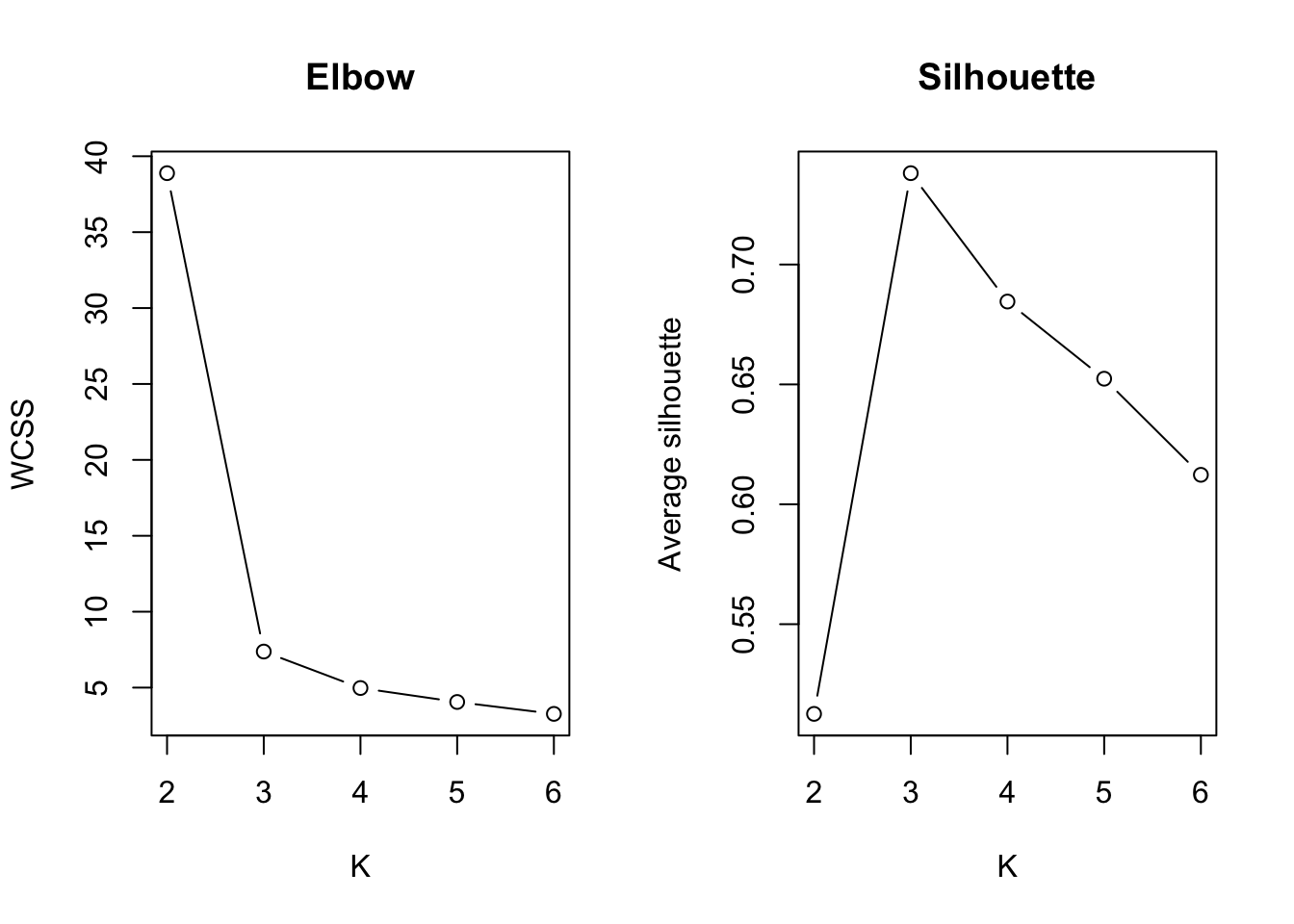
Elbow. Plot WCSS against K. WCSS falls mechanically as K grows — even structureless data can show a bend. A visible bend is a shortlist cue, not proof of natural clusters.
Silhouette. For observation i, let a(i) be the average dissimilarity to other points in its own cluster, and b(i) the lowest average dissimilarity to another cluster. Then
s(i) = \frac{b(i) - a(i)}{\max\{a(i), b(i)\}}.
Long positive bar: secure assignment.
Near zero: borderline.
Negative: another cluster is closer on average.
Worked value.a(i)=1.20, b(i)=1.50 gives s(i)=(1.50-1.20)/\max(1.20,1.50)=0.20. Mildly positive — not a strong assignment. Follow up by inspecting that observation’s neighbours or the silhouette plot.
Gap. The gap statistic compares observed WCSS with WCSS from reference data that have no cluster structure. A large positive gap means the fitted groups are more compact than the no-structure reference. Course workflow: shortlist candidates; do not stop at a single automatic rule.
2.1.5 Stability: two different questions
Reproducibility across seeds with a fixed nstart asks whether random initialisation is the weak point.
Agreement across 90% subsamples asks whether the result is sensitive to which observations are present.
Both can look good for different reasons. Seed stability does not cancel subsample fragility.
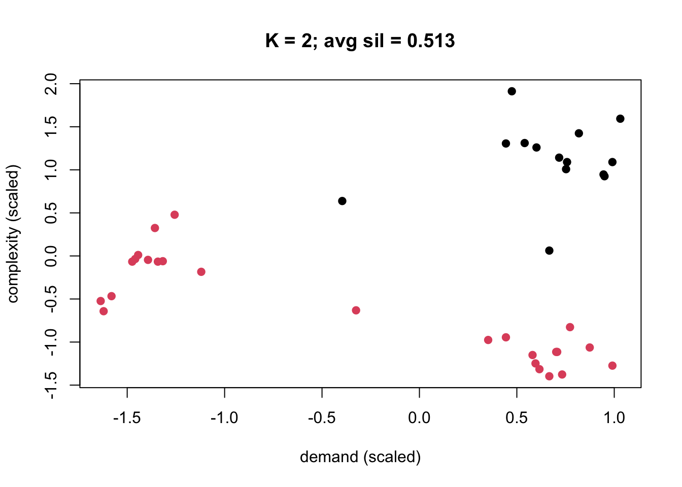
plot(x, col = fits[[1]]$cluster, pch =19,xlab ="demand (scaled)", ylab ="complexity (scaled)",main =paste("K = 2; avg sil =", round(avg_sil[1], 3)))
Partition at K = 2.
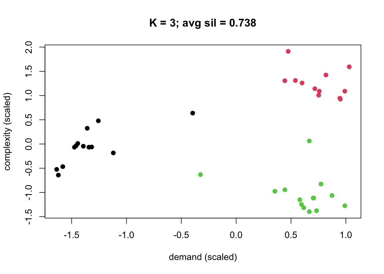
plot(x, col = fits[[2]]$cluster, pch =19,xlab ="demand (scaled)", ylab ="complexity (scaled)",main =paste("K = 3; avg sil =", round(avg_sil[2], 3)))
Partition at K = 3.
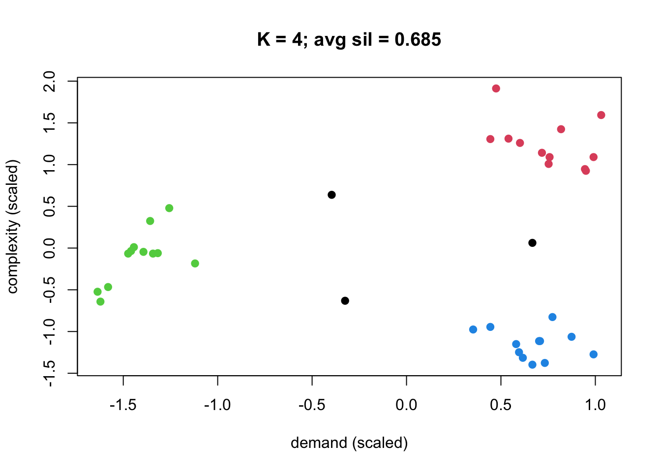
plot(x, col = fits[[3]]$cluster, pch =19,xlab ="demand (scaled)", ylab ="complexity (scaled)",main =paste("K = 4; avg sil =", round(avg_sil[3], 3)))
Partition at K = 4.
A falling WCSS alone does not pick K. Compare silhouette, negative counts, stability, and whether the profiles would change a decision.
2.1.8 Not examinable
K-medoids / PAM (Lecture 1–2, slides 24–32): medoids are actual observations; PAM minimises total dissimilarity to medoids. Name them if asked what was excluded. Do not revise the algorithm for this exam.
2.2 Reference
The best achievable WCSS is non-increasing in K. A single fitted run can still show a higher WCSS at a larger K if that run hit a poorer local optimum.
Duplicating a feature is like overweighting it in the distance (roughly multiplying its contribution).
Uniform scaling of one feature changes the solution; translating or rotating all points together does not change Euclidean k-means geometry in the same way.
Course workflow shortlists K from elbow / silhouette / gap disagreement, then compares assignments, stability, profiles, and usefulness.
Gap one-standard-error rule: choose the smallest K whose gap is within one SE of the maximum gap (as in the exercise set table).
2.3 Recall
Official — B1 (one iteration)
Six points A–F as in the exercise set. Start at \boldsymbol{\mu}_1=A=(1,1), \boldsymbol{\mu}_2=D=(7,7). Assign, then update.
Answer
Assign: \{A,B,C\} to 1, \{D,E,F\} to 2. Updated centroids: (4/3,4/3) and (22/3,22/3). Reason: nearest-centroid assignment, then cluster means.
Official — B3 (silhouette)
a(i)=1.20, b(i)=1.50. Compute s(i) and interpret.
Answer
s(i)=0.20. Mildly positive: own cluster is closer, but not by much. Follow up: inspect the observation on a silhouette plot or compare distances to the competing cluster.
Official-style MCQ — nstart
What does kmeans(x, centers = 4, nstart = 25) do with set.seed set?
Answer
Seed makes the random process repeatable; nstart = 25 tries several initialisations and retains a lowest-WCSS solution among them. It does not guarantee the global optimum.
Official-style — negative silhouette
What does a negative silhouette say most directly?
Answer
The nearest alternative cluster is closer on average than the assigned cluster.
Original — seed vs subsample
A partition is identical across 100 seeds with nstart = 25, but changes across 90% subsamples. What does that say?
Answer
Initialisation is not the main weak point; the clustering is sensitive to which observations are present. Seed reproducibility alone is not enough.