set.seed(5077)
n <- 400
t <- runif(n, 0, 3 * pi)
h <- runif(n, 0, 20)
swiss <- cbind(x = t * cos(t), y = h, z = t * sin(t))
cols <- hcl.colors(n, "Zissou 1")[rank(t)]6 ISOMAP
Study time: about 2 hours. Classical MDS on approximate geodesic (graph) distances.
6.1 Pass
6.1.1 Situation
Euclidean distance cuts through empty space. On a Swiss roll, two points can be close in ambient \mathbb{R}^3 yet far apart along the rolled sheet. The sheet is intrinsically two-dimensional: position along the roll and height.
ISOMAP replaces straight-line distances with distances that travel along the data cloud, then runs classical MDS.
6.1.2 Algorithm
- Compute ordinary Euclidean distances between observations.
- Build a neighbourhood graph: k-nearest neighbours, or an \varepsilon-ball.
- Replace pairwise distances by shortest-path lengths on that graph (approximate geodesics).
- Apply classical MDS to the graph-distance matrix.
Classical MDS is used because it is fast and the non-linearity is already handled by the distances. True continuous geodesics are not computed — only graph shortest paths.
6.1.3 Neighbourhood size
- k=1: graph often disconnected; some shortest paths do not exist.
- k=n-1: complete graph; shortest path is the direct Euclidean edge → ISOMAP collapses toward classical MDS (and toward PCA when inputs are Euclidean feature distances).
- Reasonable k: large enough for connectivity, small enough to avoid short-circuit edges that jump across the roll.
Noise is dangerous: a noisy point in empty space can bridge regions that should stay far apart on the manifold.
k-NN adapts when density varies (every point gets neighbours). An \varepsilon-graph needs a trusted maximum edge length and roughly uniform density.
6.1.4 Interactive check: three neighbourhoods
fit5 <- vegan::isomap(dist(swiss), ndim = 2, k = 5)
plot(vegan::scores(fit5), col = cols, pch = 16,
     xlab = "ISOMAP1", ylab = "ISOMAP2", main = "k = 5")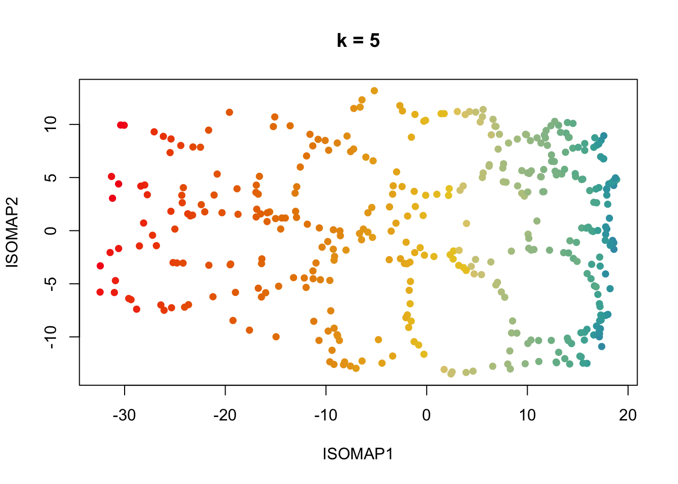
fit15 <- vegan::isomap(dist(swiss), ndim = 2, k = 15)
plot(vegan::scores(fit15), col = cols, pch = 16,
     xlab = "ISOMAP1", ylab = "ISOMAP2", main = "k = 15")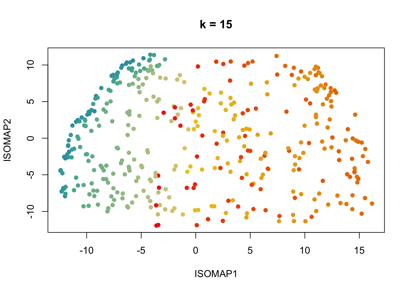
fit40 <- vegan::isomap(dist(swiss), ndim = 2, k = 40)
plot(vegan::scores(fit40), col = cols, pch = 16,
     xlab = "ISOMAP1", ylab = "ISOMAP2", main = "k = 40")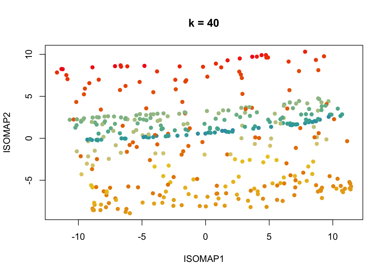
Successful unfolding keeps the colour (the roll parameter) changing smoothly across the plane. PCA on the same points cannot unroll the sheet — it only sees linear projections.
6.1.5 Commands
Course demo (vegan):
fit <- vegan::isomap(dist(x), ndim = 2, k = 12)
coords <- vegan::scores(fit)
Last year’s blank (Rdimtools):
iso <- Rdimtools::do.isomap(x, ndim = 2, type = c("knn", 15))
plot(iso$Y, pch = 16)
Know both extraction patterns: scores(fit) versus $Y.
6.2 Reference
- Failure modes: disconnected graphs, short-circuit edges, uneven density, outliers, multiple manifolds.
- ISOMAP does not give loadings or a decoder back to features.
- Graph distance example questions: sum edge weights along the shortest path (see slide example if a figure is provided in the paper).
6.3 Recall
Official — why classical MDS
Why classical rather than non-metric MDS inside ISOMAP?
Answer
Classical MDS is faster; non-linearity is already in the graph distances.
Official — geodesic?
Does ISOMAP use geodesic distances?
Answer
Approximately: shortest paths on a neighbourhood graph, not continuous geodesics on the manifold.
Official — k extremes
Effect of k=1 vs k=n-1?
Answer
k=1: often disconnected. k=n-1: reduces to classical MDS on Euclidean edges.
Official — Swiss roll
In what sense is the Swiss roll 2-D in 3-D?